1. Overview
In the previous article, I’ve explained in detail on how to implement screen space reflections technique using the linear tracing method and also showed how the method can be optimized using a couple of techniques. Here is the link to the article.
In this article, I’d like to introduce a different tracing method that greatly outperforms the linear tracing method while maintaining accuracy. The method is called ‘HI-Z Tracing’ method.
This method was first introduced in the chapter, ‘Hi-Z Screen-Space Cone-Traced Reflections by Yasin Uludag’, in the book, ‘GPU PRO 5’. Even though I bought this book many years ago and I did read the chapter when I bought it, I haven’t tried to implement it myself until recently.
Okay. If there is already a book for explaining this technique, what’s the point me writing this article?
First, the book doesn’t explain the technique completely. It doesn’t come with a full source code. It does provide the source code for the main body while the code for the functions called from the main body are missing. Even the code for the main body appears to have couple of typos. And, the book doesn’t give you instructions how to implement those missing functions. it’s all the reader’s job to fill the missing parts. So, in this article, I’m going to give you the full detail of how this technique can be implemented. Also, I’m sharing the full source code of my implementation which can be found here.
Second, the method explained in the book comes with a couple of limitations. First, it works only for screen resolutions of power of 2. Most of the resolutions used in video games such as 1920×1080 are not power of 2. So, it will be useless if the technique can’t be used with non-power of 2 resolutions. Second, I found out that the accuracy of the method decreases depending on the direction of the reflection ray. It works great when the ray moves primarily away from the camera ( in other word, |dir.z| >> |dir.xy| ). However, it loses accuracy when the ray moves primarily in horizontal or vertical directions ( in other word, |dir.xy| >> |dir.z| ). Third, the method introduced in the book only works when the reflection ray is moving away from the camera. In other word, the method doesn’t work when the reflection is moving toward the camera. I’ve managed to find solutions that can overcome these limitations. So, I’m going to talk about that.
Third, I found the technique really fantastic. So, by writing this article, I hope I spread this technique to more and more people and help them take advantage of it whenever possible.
2. Overview of the HI-Z Tracing Method
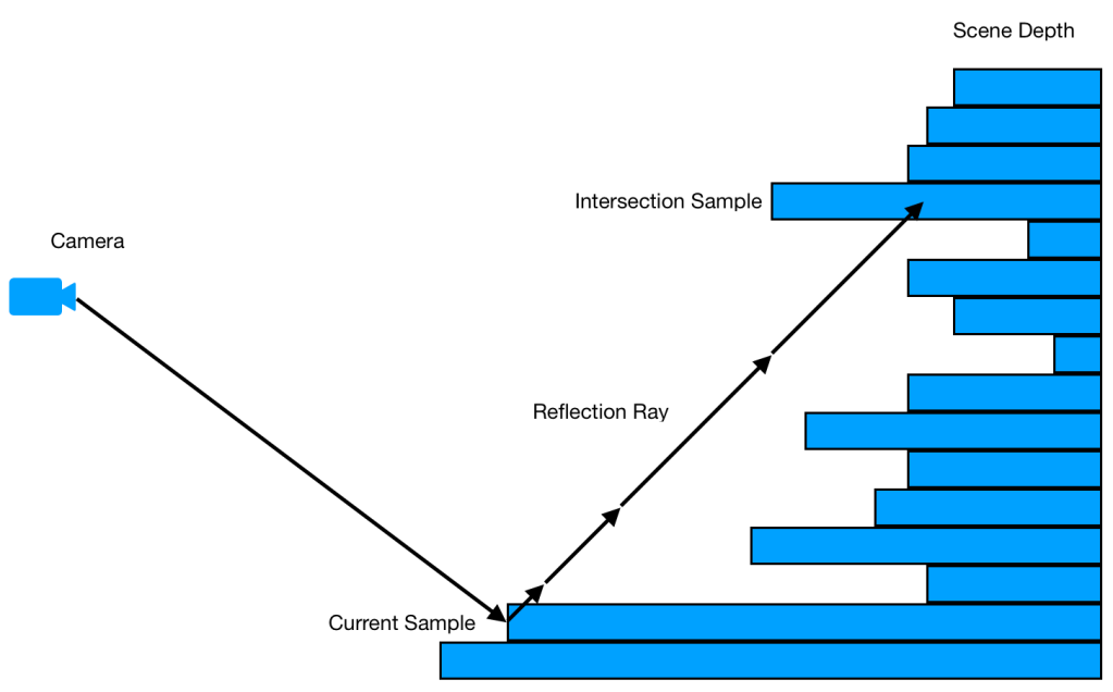
Let me first show you what the problem is in the linear tracing that we want to improve using the Hi-Z tracing. Below image depicts how a ray is traced in the linear tracing.

In order to reach the intersection sample, it has to stop at every single sample between the starting sample and the intersection sample and do a depth comparison. But, one can notice that for majority of the time, the ray is just moving in an empty space without any hits. So, the question is, is there a way to skip the empty space more quickly? The answer is the Hi-Z tracing.
The Hi-Z tracing method creates an acceleration structure called Hi-Z buffer ( or texture ). The structure is essentially a quad tree of the scene depth where each cell in a quad tree level is set to be the minimum (or maximum depending on the z axis direction) of the 4 cells in the above level as below.
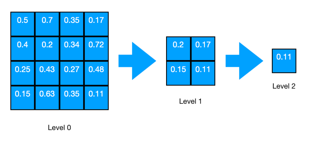
It creates the levels from the full resolution all the way down to 1×1. It uses mip levels of a texture to store each quad tree level and access them.
Below image gives you an idea of what it looks like when traced with hi-z tracing using the structure. Compare it with the picture of linear tracing above.
As can be seen in the picture, it stops at fewer samples before it reaches the intersection. This is how this method is capable of outperforming the linear tracing method.
So, naturally, the method is divided into two passes. In the first pass, it generates the hi-z texture using the scene depth texture as the base level. In the second pass, it runs the SSR using the hi-z texture from the previous pass.
3. The Hi-Z pass
In this pass, we are constructing the acceleration structure called the Hi-Z texture which will be used in the subsequent SSR pass. This pass is comprised of number of sub-passes where each sub-pass generates each level of the quad tree and stores in the mipmaps of the Hi-Z texture.
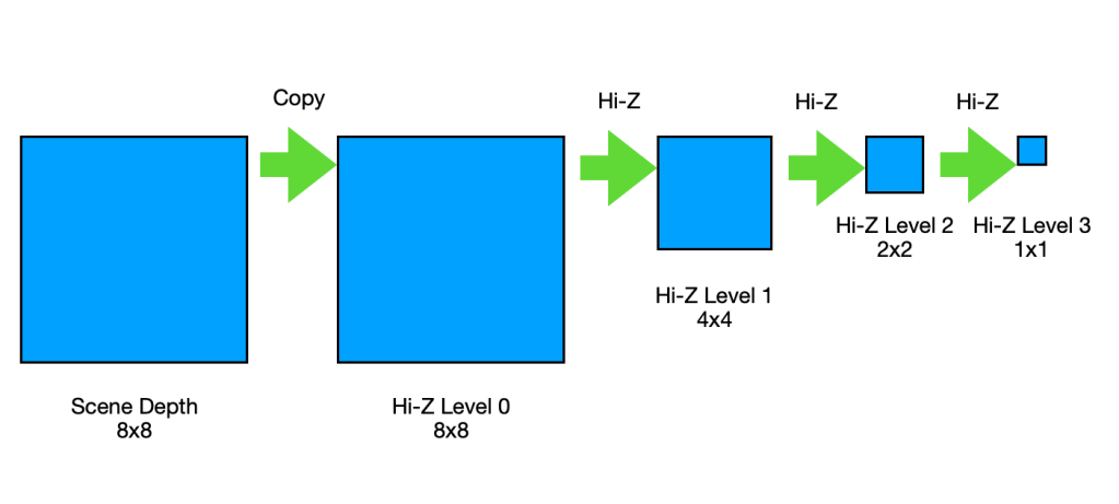
The first sub-pass generates the base level of the Hi-Z texture by just copying the scene depth texture to the level 0 mip of the Hi-Z texture.
And then, number of sub-passes follows where each sub-pass generates the next mip level using the previous mip level as the input using the hi-z generation compute kernel and it finishes when the last mip of 1×1 size is generated. The diagram below describes how these sub-passes work.
According to the book, each cell in a level is set to the minimum of 2×2 cells in the above level as below.
And, that could be implemented as below.
kernel void kernel_createHiZ(texture2d<float, access::read> depth [[ texture(0) ]],
                           texture2d<float, access::write> outDepth [[ texture(1) ]],
                                  uint2 tid [[thread_position_in_grid]])
{
    uint2 vReadCoord = tid<<1;
    uint2 vWriteCoord = tid;

    float4 depth_samples = float4(
                                  depth.read(vReadCoord).x,
                                  depth.read(vReadCoord + uint2(1,0)).x,
                                  depth.read(vReadCoord + uint2(0,1)).x,
                                  depth.read(vReadCoord + uint2(1,1)).x
                                  );

    float min_depth = min(depth_samples.x, min(depth_samples.y, min(depth_samples.z, depth_samples.w)));

    outDepth.write(float4(min_depth), vWriteCoord);
}
However, this method only works when the dimension of the above level is multiple of 2 of the dimension of the current level which can happen when the screen resolution is not power of 2. See how the code above generates the cells in level 1 when the dimension of level 0 is 5×5.

If you look at the cells in level 1, you could notice that it failed to take the cells at the bottom edge and the right edge in level 0 into account when generating level 1. So, clearly, this implementation doesn’t work when the dimension is not multiple of 2. Then, how can we correct it?
To find a correct solution, let’s visualize the area in level 0 covered by each cell in level 1.
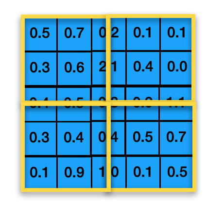
Each yellow box corresponds to the area covered by each cell in level 1. As can be seen in the image, each cell in level 1 covers 2.5×2.5 cells instead of 2×2 cells in level 0. Therefore, when the dimension of the above level is not multiple of 2, the cells need to be set to the minimum of 3×3 cells. And, the code below shows the implementation with the fix.
kernel void kernel_createHiZ(texture2d<float, access::read> depth [[ texture(0) ]],
                           texture2d<float, access::write> outDepth [[ texture(1) ]],
                                  uint2 tid [[thread_position_in_grid]])
{
	float2 depth_dim = float2(depth.get_width(), depth.get_height());
	float2 out_depth_dim = float2(outDepth.get_width(), outDepth.get_height());

	float2 ratio = depth_dim / out_depth_dim;

	uint2 vReadCoord = tid<<1;
        uint2 vWriteCoord = tid;

        float4 depth_samples = float4(
                                  depth.read(vReadCoord).x,
                                  depth.read(vReadCoord + uint2(1,0)).x,
                                  depth.read(vReadCoord + uint2(0,1)).x,
                                  depth.read(vReadCoord + uint2(1,1)).x
                                  );

        float min_depth = min(depth_samples.x, min(depth_samples.y, min(depth_samples.z, depth_samples.w)));

	bool needExtraSampleX = ratio.x>2;
        bool needExtraSampleY = ratio.y>2;

        min_depth = needExtraSampleX ? min(min_depth, min(depth.read(vReadCoord + uint2(2,0)).x, depth.read(vReadCoord + uint2(2,1)).x)) : min_depth;
        min_depth = needExtraSampleY ? min(min_depth, min(depth.read(vReadCoord + uint2(0,2)).x, depth.read(vReadCoord + uint2(1,2)).x)) : min_depth;
        min_depth = (needExtraSampleX && needExtraSampleY) ? min(min_depth, depth.read(vReadCoord + uint2(2,2)).x) : min_depth;

        outDepth.write(float4(min_depth), vWriteCoord);
}
4. The SSR pass with Hi-Z Tracing
Now that we have the Hi-Z texture created in the previous pass, we can now move on to the fun part, the SSR pass with Hi-Z tracing.
For this pass, we’ll use the same code for the main body as the code we used for the linear tracing method. The only difference is that it takes Hi-Z texture instead of Scene Depth texture as input. And, it calls ‘FindIntersection_HiZ’ instead of ‘FindIntersection_Linear’ for tracing a ray. Below is the code.
kernel void kernel_screen_space_reflection_hi_z(texture2d<float, access::sample> tex_normal_refl_mask [[texture(0)]],
                                                texture2d<float, access::sample> tex_hi_z [[texture(1)]],
                                                texture2d<float, access::sample> tex_scene_color [[texture(2)]],
                                                texture2d<float, access::write> tex_output [[texture(3)]],
                                                const constant SceneInfo& sceneInfo [[buffer(0)]],
                                                uint2 tid [[thread_position_in_grid]])
{
    float4 finalColor = 0;

    float4 NormalAndReflectionMask = tex_normal_refl_mask.read(tid);
    float4 color = tex_scene_color.read(tid);
    float4 normalInWS = float4(normalize(NormalAndReflectionMask.xyz), 0);
    float3 normal = (sceneInfo.ViewMat * normalInWS).xyz;
    float reflection_mask = NormalAndReflectionMask.w;

    float4 skyColor = float4(0,0,1,1);

    float4 reflectionColor = 0;
    if(reflection_mask != 0)
    {
	reflectionColor = skyColor;
        float3 samplePosInTS = 0;
        float3 vReflDirInTS = 0;
        float maxTraceDistance = 0;
        // Compute the position, the reflection vector, maxTraceDistance of this sample in texture space.
        ComputePosAndReflection(tid, sceneInfo, normal, tex_hi_z, samplePosInTS, vReflDirInTS, maxTraceDistance);

        // Find intersection in texture space by tracing the reflection ray
        float3 intersection = 0;
        float intensity = FindIntersection_HiZ(samplePosInTS, vReflDirInTS, maxTraceDistance, tex_hi_z, sceneInfo, intersection);

        // Compute reflection color if intersected
	reflectionColor = ComputeReflectedColor(intensity,intersection, skyColor, tex_scene_color);
    }

    // Add the reflection color to the color of the sample.
    finalColor = color + reflectionColor;

    tex_output.write(finalColor, tid);
}
I’ve already talked about this part of the code in the previous article for linear tracing. So, let’s just skip this one and jump into the function, ‘FindIntersection_HiZ’ where it uses Hi-Z tracing to find an intersection.
float FindIntersection_HiZ(float3 samplePosInTS,
                         float3 vReflDirInTS,
                          float maxTraceDistance,
                         texture2d<float, access::sample> tex_hi_z,
                         const constant SceneInfo& sceneInfo,
                         thread float3& intersection)
{
    const int maxLevel = tex_hi_z.get_num_mip_levels()-1;

    float2 crossStep = float2(vReflDirInTS.x>=0 ? 1 : -1, vReflDirInTS.y>=0 ? 1 : -1);
    float2 crossOffset = crossStep / sceneInfo.ViewSize / 128;
    crossStep = saturate(crossStep);

    float3 ray = samplePosInTS.xyz;
    float minZ = ray.z;
    float maxZ = ray.z + vReflDirInTS.z * maxTraceDistance;
    float deltaZ = (maxZ - minZ);

    float3 o = ray;
    float3 d = vReflDirInTS * maxTraceDistance;

    int startLevel = 2;
    int stopLevel = 0;
    float2 startCellCount = getCellCount(startLevel, tex_hi_z);

    float2 rayCell = getCell(ray.xy, startCellCount);
    ray = intersectCellBoundary(o, d, rayCell, startCellCount, crossStep, crossOffset*64);

    int level = startLevel;
    uint iter = 0;
    bool isBackwardRay = vReflDirInTS.z<0;
    float rayDir = isBackwardRay ? -1 : 1;

    while(level >=stopLevel && ray.z*rayDir <= maxZ*rayDir && iter<sceneInfo.maxIteration)
    {
        const float2 cellCount = getCellCount(level, tex_hi_z);
        const float2 oldCellIdx = getCell(ray.xy, cellCount);

        float cell_minZ = getMinimumDepthPlane((oldCellIdx+0.5f)/cellCount, level, tex_hi_z);
        float3 tmpRay = ((cell_minZ > ray.z) && !isBackwardRay) ? intersectDepthPlane(o, d, (cell_minZ - minZ)/deltaZ) : ray;

        const float2 newCellIdx = getCell(tmpRay.xy, cellCount);

        float thickness = level == 0 ? (ray.z - cell_minZ) : 0;
        bool crossed = (isBackwardRay && (cell_minZ > ray.z)) || (thickness>(MAX_THICKNESS)) || crossedCellBoundary(oldCellIdx, newCellIdx);
        ray = crossed ? intersectCellBoundary(o, d, oldCellIdx, cellCount, crossStep, crossOffset) : tmpRay;
        level = crossed ? min((float)maxLevel, level + 1.0f) : level-1;

        ++iter;
    }

    bool intersected = (level < stopLevel);
    intersection = ray;

    float intensity = intersected ? 1 : 0;

    return intensity;
}
This is the main body for the tracing function. Not so much complicated than the linear tracing method, isn’t it?
Let’s get to each section.
    const int maxLevel = tex_hi_z.get_num_mip_levels()-1;

    float2 crossStep = float2(vReflDirInTS.x>=0 ? 1 : -1, vReflDirInTS.y>=0 ? 1 : -1);
    float2 crossOffset = crossStep / sceneInfo.ViewSize / 128;
    crossStep = saturate(crossStep);
Here, it sets maxLevel which is just the level of the last mip in the Hi-Z texture.
Next, it sets two variables, ‘crossStep’ and ‘crossOffset’. These two variables are used to move the ray to the next cell in the grid of the quad tree. Here, the my code for setting ‘crossOffset’ is slightly different from the code in the book. In the book, ‘crossOffset’ is set using this code below.
crossOffset.xy = crossStep.xy * HIZ_CROSS_EPILSON.xy;It’s almost identical to my code. But the problem is that the book completely misses to explain how exactly ‘HIZ_CROSS_EPILSON’ is calculated. So, I had to come up with my own formula for that. ‘crossOffset’ is used to push a ray by a tiny amount of distance to make sure the ray is in the next cell after doing a cell crossing. (As for the cell crossing, we’ll talk more about it later.). So, I thought ‘sceneInfo.ViewSize / 128’ is a reasonable value for that purposes.
    float3 ray = samplePosInTS.xyz;
    float minZ = ray.z;
    float maxZ = ray.z + vReflDirInTS.z * maxTraceDistance;
    float deltaZ = (maxZ - minZ);
In the next part, it initializes the ray to the position of the current sample in texture space. Then, it sets ‘minZ’ and ‘maxZ’ which are the minimum and the maximum position of the ray in z axis. This is the range in z axis where we will trace the ray within. Then, it sets ‘deltaZ’ to be the distance between minZ and maxZ.
    float3 o = ray;
    float3 d = vReflDirInTS * maxTraceDistance;
Next, it sets ‘o’ and ‘d’. This is another point where my code differs from the original code in the book. The two variables, ‘o’ and ‘d’ are used to parameterize position of reflection ray using depth as parameter.
Let me first show you how it is parameterized in the book. Then, I’ll explain the problem with that method and my solution for that.
In the book, ‘o’ is set to the point along the reflection direction where z component is 0 which puts the position on the near plane of the camera. And, ‘d’ is set so that when added it to ‘o’, it moves ‘o’ along the reflection direction to the point where z component is 1 which puts the position on the far plane of the camera. Below image illustrates the idea.

Using o and d, we can use the equation below to get the position of any point along the ray using depth as parameter.
ray(depth) = o + d * depth
Using this equation, when depth is 0, ray becomes ‘o’ and when depth is 1, ray becomes (o+d). To get the position of the ray origin, we just need to plugin the depth at the origin of the ray ( in other word, the depth of the current sample).
So, what is the problem with this approach? The problem is that, depending on the direction of the reflection ray, while the z component of them are always 0 and 1, the xy components of ‘o’ and ‘d’ can go really really large ( positive or negative ). And, that can cause precision problems as we are using 32 bit float to represent the numbers. See the image below as an example.
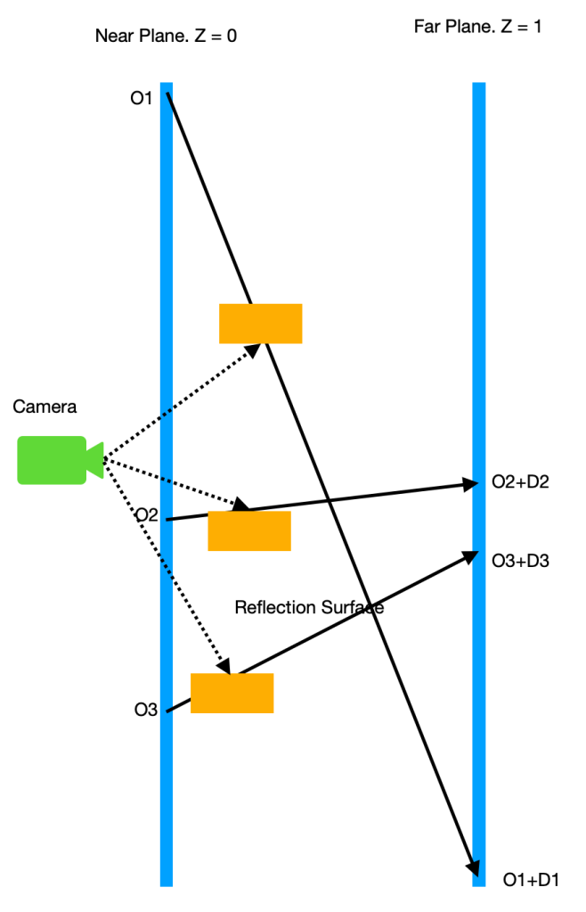
In this example, we can see that, as the x or y component of reflection direction gets larger than the z component, the position of ‘o’ moves further away from the center of view and the length of ‘d’ gets longer which makes the magnitude of ‘o’ and ‘d’ increase.
It is very important to keep the magnitude of ‘o’ and ‘d’ as small as possible to minimize the precision problem. So, here is my solution to minimize the problem.
First, I’m going to set ‘o’ to be the origin of the ray because we’ll never trace the ray behind the origin.
Second, I’m going to set ‘d’ in a way that (o+d) is the maximum trace point where the maximum trace point is a point along the ray right before it goes out of visible boundary. Again, this is fine because we’ll never need to trace the ray after the ray goes out of visible boundary. We have already calculated where this point is. And, the point is stored in ‘maxTraceDistance’ as the distance from the ray origin to the maximum trace point.
With this solution, the example above changes to this.

With this solution, the magnitude of xyz components in o and d will never exceed 1. And, this will help minimize precision problems when using o and d in the equations later.
Okay. Now, let’s move on to the next section.
    int startLevel = 2;
    int stopLevel = 0;
Here, we set ‘startLevel’ and ‘stopLevel’. startLevel is the level in the Hi-Z quad tree that we will start tracing the ray in. stopLevel is the level in the Hi-Z quad tree that we will stop tracing the ray when the current level is higher than stopLevel. We’ll see how these numbers are used in the subsequent sections.
    float2 startCellCount = getCellCount(startLevel, tex_hi_z);

    float2 rayCell = getCell(ray.xy, startCellCount);
    ray = intersectCellBoundary(o, d, rayCell, startCellCount, crossStep, crossOffset*64, minZ, maxZ);
In this section of the code, the goal is to move the current ray to the next cell in the reflection direction to avoid ‘self-intersection’.
The function ‘getCellCount’ returns the number of cells in the quad tree at the given level. It is implemented as below.
float2 getCellCount(int mipLevel, texture2d<float, access::sample> tex_hi_z)
{
    return float2(tex_hi_z.get_width(mipLevel) ,tex_hi_z.get_height(mipLevel));
}
So, cell count is just the resolution of the Hi-Z texture at the specific mip level where the mip level corresponds to the quad tree level.
The function ‘getCell’ returns the 2D integer index of the cell that contains the given 2D position within it. It takes ‘pos’ and ‘cell_count’ as input. ‘pos’ is the position to find the cell for. ‘cell_count’ is width and height of the quad tree level to find the cell for. The code is below.
float2 getCell(float2 pos, float2 cell_count)
{
    return float2(floor(pos*cell_count));
}
So, with getCellCount(), we can get the cell count of the quad tree at the start level. Then, using that cell count, we can call getCell to get the cell index of the current ray on the quad tree at the start level.
Now, we have the current cell index that the ray is on. Next, we’ll use ‘intersectCellBoundary’ to push the ray to the right next to the current cell. So, after this, the ray will be on the next cell but still very close to the boundary between the current cell and the next cell. Below image shows what this function does.

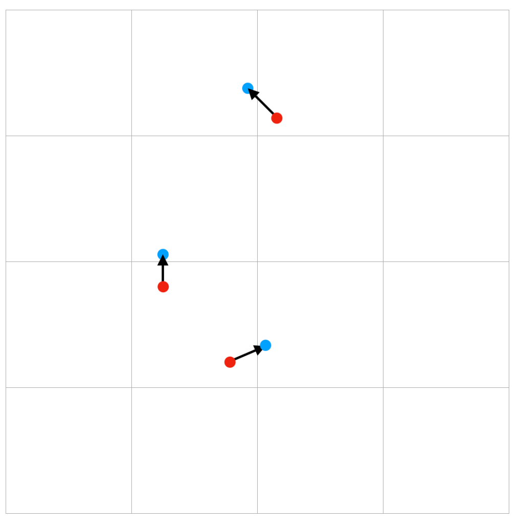
The red dots represent the current position. And, the blue dots represents the new positions calculated using ‘intersectCellBoundary’. The arrows represents the direction of the reflection ray.
Below is the code for the function.
float3 intersectCellBoundary(float3 o, float3 d, float2 cell, float2 cell_count, float2 crossStep, float2 crossOffset)
{
	float3 intersection = 0;

	float2 index = cell + crossStep;
	float2 boundary = index / cell_count;
	boundary += crossOffset;

	float2 delta = boundary - o.xy;
	delta /= d.xy;
	float t = min(delta.x, delta.y);

	intersection = intersectDepthPlane(o, d, t);

	return intersection;
}
This function is where crossStep and crossOffset are being used. crossStep is added to the current cell to get the next cell index. By dividing the cell index by cell count, we can get the position of the boundaries between the current cell and the new cell . Then, crossOffset is used to push the position just a tiny bit further to make sure the new position is not right on the boundary.
Then the delta between the new position and the origin is calculated. The delta is divided by xy component of ‘d’ vector. After the division, the x and y component in delta will have value between 0 to 1 which represents how far the delta position is from the origin of the ray.
Then, we take the minimum of the two components, x and y of delta because we want to cross the nearest boundary. Then, we can finally call ‘intersectDepthPlane’ to calculate the new position.
float3 intersectDepthPlane(float3 o, float3 d, float z)
{
	return o + d * z;
}
This function is just the parameterized form for calculating position on the reflection ray that I introduced earlier.
By the way, the code in the book for pushing the start position to the next cell is this.
ray = intersectCellBoundary(o, d, rayCell, startCellCount, crossStep, crossOffset);The only difference between the code in the book and the code in my implementation is that my implementation multiplies 64 to ‘crossOffset’ when calling intersectCellBoundary. This multiplication was necessary to properly push the ray to the next cell when the screen resolution is not power of 2. Why is it necessary ?
I found out that ,without the multiplication and when startLevel is larger than 0, it’s possible that calling ‘intersectCellBoundary’ to push the ray to the next cell does move the ray to the next cell in the start level but not in the levels above of the start level. See below for example.
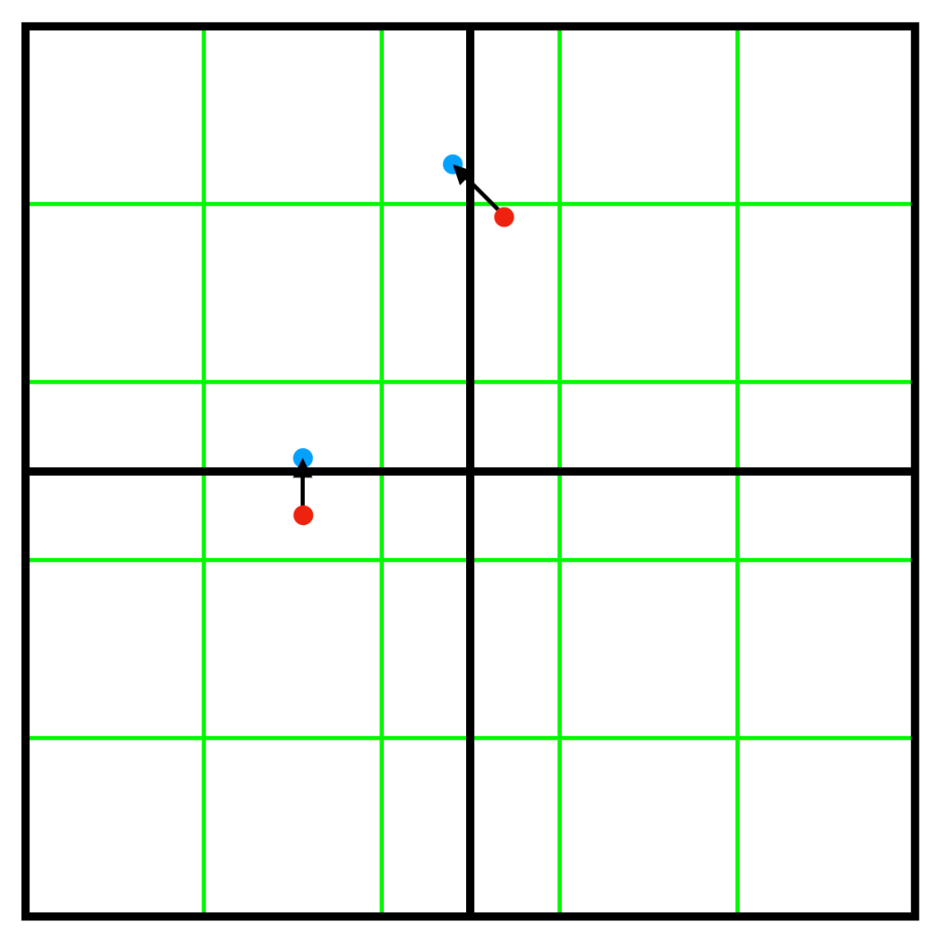
The level with green cells are 5×5. The level with black cells are 2×2. Two positions are pushed to the next cell. While the one at the top did work correctly, the one at the middle didn’t do quite well. It did move the position to the next cell of 2×2 level. But, it failed to move the position to the next cell of 5×5 level. This problem doesn’t happen when the screen resolution is power of 2.
Using a bigger crossOffset does help fix this problem by moving the position further away from the boundary. So, that’s why I ended up multiplying 64 to crossOffset.
All right. Now, we can move to the next part where we actually trace the ray.
    int level = startLevel;
    uint iter = 0;
    bool isBackwardRay = vReflDirInTS.z<0;
    float rayDir = isBackwardRay ? -1 : 1;

    while(level >=stopLevel && ray.z*rayDir <= maxZ*rayDir && iter<sceneInfo.maxIteration)
    {
        const float2 cellCount = getCellCount(level, tex_hi_z);
        const float2 oldCellIdx = getCell(ray.xy, cellCount);

        float cell_minZ = getMinimumDepthPlane((oldCellIdx+0.5f)/cellCount, level, tex_hi_z);
        float3 tmpRay = ((cell_minZ > ray.z) && !isBackwardRay) ? intersectDepthPlane(o, d, (cell_minZ - minZ)/deltaZ) : ray;

        const float2 newCellIdx = getCell(tmpRay.xy, cellCount);

        float thickness = level == 0 ? (ray.z - cell_minZ) : 0;
        bool crossed = (isBackwardRay && (cell_minZ > ray.z)) || (thickness>(MAX_THICKNESS)) || crossedCellBoundary(oldCellIdx, newCellIdx);
        ray = crossed ? intersectCellBoundary(o, d, oldCellIdx, cellCount, crossStep, crossOffset) : tmpRay;
        level = crossed ? min((float)maxLevel, level + 1.0f) : level-1;

        ++iter;
    }
Let’s follow the code to see what it does.
First, it starts a while loop. The exit condition is when the current level is higher than stop level or z position of the ray goes beyond maxZ. We also limit the number of iterations by ‘maxIteration’.
In the loop, first, it gets the cell count of the current level. Then, it gets the cell index of the current ray on the current level.
Then, it obtains the minimum depth of the current cell in the current quad tree level using ‘getMinimumDepthPlane’ which is implemented as below.
float getMinimumDepthPlane(float2 p, int mipLevel, texture2d<float, access::sample> tex_hi_z)
{
	constexpr sampler pointSampler(mip_filter::nearest);
	return tex_hi_z.sample(pointSampler, p, level(mipLevel)).x;
}
The function just simply samples the Hi-Z texture at the given sample position at the given mip level.
And, here is another place where my implementation slightly differs from the book. Below is the code in the book.
float minZ = getMinimumDepthplane(ray.xy, level, rootLevel);Now, the book doesn’t provide how ‘getMinimumDepthplane’ is implemented. So, I have no idea how the three parameters are actually used. But, if I’m right, it would probably use ‘ray.xy’ as the sampling coordinate and ‘level’ as the mip level. And, I have no idea what the use of ‘rootLevel’ might be.
So, at first, I tried the same approach where I use ‘ray.xy’ to sample from the texture. But, it turns out that doing that sometimes results in sampling incorrect position in the texture. My guess is that it’s because sometimes ray.xy lies right at the boundary between two samples and when I’m unlucky I get the wrong side of the sample.
So, instead of using ray.xy as the sampling coordinate, I used the cellIndex to calculate the position of the center of the current cell. And then, I used that position to sample from the texture. And that resolved the problem of incorrect sampling completely.
Okay. Once the minimum depth of the current cell is obtained through ‘getMinimumDepthPlane’, we need to compare the min depth with the current depth of the ray. There can be two outcomes from the comparison.
A. current depth >= min depth : This means the ray is inside of the volume of the current cell. If the current level is the first level, then we have found an intersection. But, if the current level is not the first level, we don’t know yet if the ray has really intersected anything. To determine that, we need to go back to the above level all the way up to the first level.
B. current depth < min depth : This means the ray is outside of the volume of the current cell. In this case, we can move the ray further to the position where the z of the new position is the min depth.

And, this is what the code below is doing.
float3 tmpRay = ((cell_minZ > ray.z) && !isBackwardRay) ? intersectDepthPlane(o, d, (cell_minZ - minZ)/deltaZ) : ray;Even when ray is moved further, the new position is stored in a temporary variable. That’s because the new position needs to be recalculated when the new position is not within the current cell.
So, that’s what the next lines of code do.
It checks if the cell index of the new position is the same as the current cell index. If not, that means the new position is on a different cell than the current cell. In that case, instead of using the new position as is, we use ‘intersectCellBoundary’ to get the position in the next cell to move the current ray to.
We also move the ray to the next cell when the thickness is thicker than ‘MAX_THICKNESS’. This is a way to allow the ray to pass through behind an object. This must be done only when the current level is 0. Otherwise, we’ll get unexpected results.
And, if the ray moved to the next cell, we move to the lower level of quad tree. If not, we move to the higher level of quad tree.
The video below illustrates how all this process works.
The black arrows and the green dots represents the position of the ray at each iteration. The red dotted lines and the red dot represents the temporary position of the ray at each iteration. The green boxes represents the cells at each quad tree level. The start level and stop level are both set to 0 in the example.
Okay. This almost concludes the loop part except there is one more detail that I want to bring up.
Everything I’ve explained so far assumes the reflection ray is moving away from camera ( moving forward). But, how does it work when the ray is moving toward camera ( moving backward) ?
This is the part where the book completely ignored to explain. But, it wasn’t that difficult to come up with my own solution for it. If you see the code, you must have noticed the variable, ‘isBackwardRay’. And, some lines of code uses this variable to handle the ray differently. As you can see, ‘isBackwardRay’ is used only in a couple of lines. And, that’s as much as you need to allow the implementation to trace the backward rays.
In the case of forward ray, the z component of the ray increases in each iteration whereas in the case of backward ray, the z decreases. That’s because a backward ray moves toward the near plane whose depth is 0. This is why the condition for terminating the loop when the ray reaches the maximum z needs to be flipped when the ray is moving backward.
And, the algorithm for tracing forward rays won’t work with backward rays. We need a new algorithm for tracing backward rays and that algorithm turns out to be even simpler than the one for forward rays.
In each iteration, we get the minimum z of the current cell. If the current ray is inside the current cell, then the ray stays and we move to the higher level. On the other hand, if the current ray is outside the current cell, we can just simply cross to the next cell and then to the lower level.
Alright. This is really everything about the loop part.
The last part is where we check if the the ray intersected or not. For that, we can check if ‘level’ is higher than ‘stopLevel’.
Also, we can set ‘intersection’ to the current position of the ray.
5. Performance comparisons with linear tracing method.
Here, I’m presenting performance comparisons between linear tracing method and Hi-Z tracing method. I’m going to run a series of comparisons where each comparison uses different max iteration count for the ray tracing loop. The loop stops either when the iteration count exceeds the max iteration or the ray reaches the maximum travel position or an intersection is found.
The GPU times were measured on my iMac Pro 2017 model where the GPU is ‘Radeon Pro Vega 64 16 GB’.
| Linear(SSR Pass) | Hi-Z(HiZ Pass + SSR Pass) | |
| MaxIteration = 1000 | 2.33ms | 1.77ms |
| MaxIteration = 300 | 1.3ms | 1.2ms |
| MaxIteration = 100 | 0.7ms | 1ms |
| MaxIteration = 25 | 0.45ms | 0.8ms |
Looking at the table, it appears that Hi-Z ran faster with MaxIteraion >= 300 while linear ran faster when MaxIteraion < 300. But, that’s not the truth. That’s because even with the same max iteration count, the Hi-Z method can trace much further than what linear method can do. See the pictures below for each max iterations.
A. MaxIteration = 1000

B. MaxIteration = 300
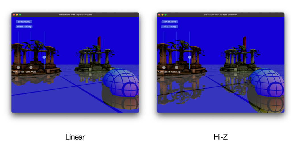
C. MaxIteration = 100
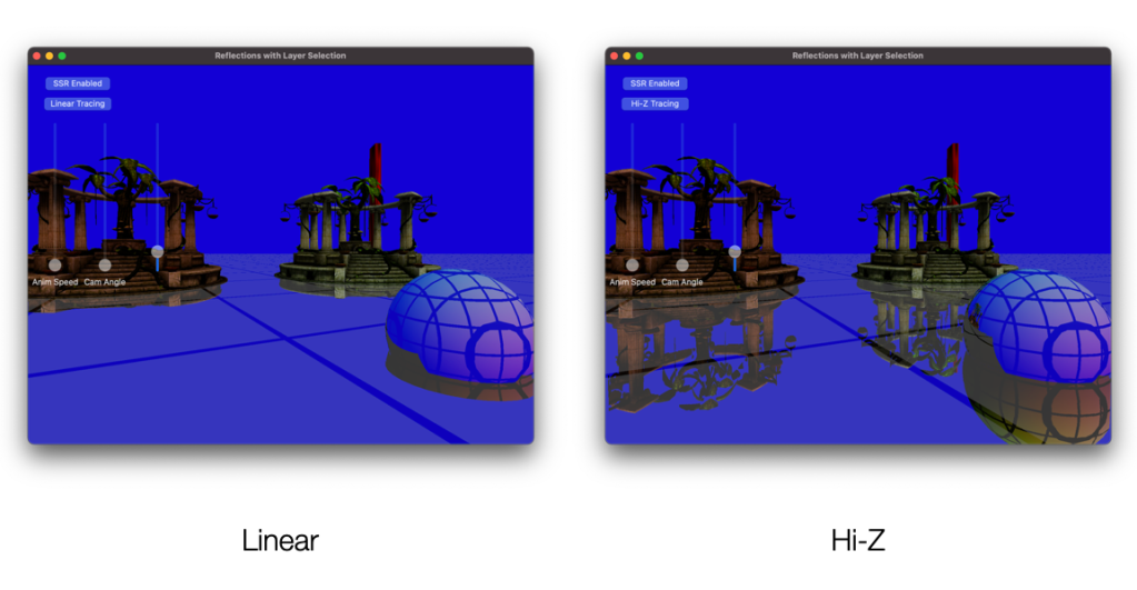
D. MaxIteration = 25
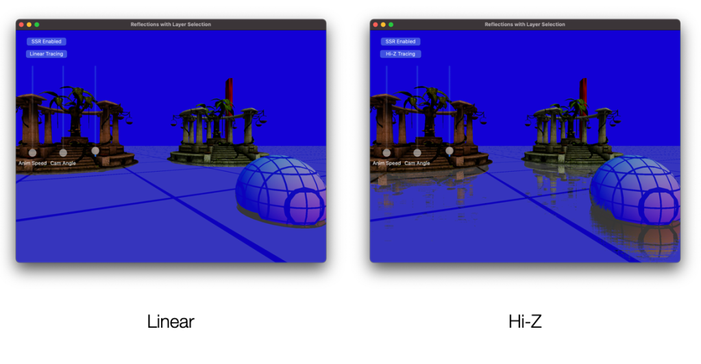
As you can see, The Hi-Z method with max iteration 100 produces result almost identical to the linear method with max iteration 1000. Now, we can see how mighty the Hi-Z tracing method is.
6. Conclusion
Starting from the instructions and code pieces presented in the book, it took some effort and time for me to get everything to work correctly in my implementation. And, I’m glad that I did.
As I said, the book doesn’t provide full detail of how to implement this technique properly. So, I hope this article help people who are interested in this technique and trying to implement it themselves.
Thanks for reading!
